Email Analytics: Charting Open Rates for Your Latest Newsletter Campaigns

An introduction to analyzing your email data using SQL and a Redshift datastore.

Using data sent to a Redshift database from Vero, we’ll put together a chart that will help you start to conceptualize how you could build out a detailed and accurate Email Dashboard for your organization.

This will also further the skills you need to analyze your email marketing data when joining it up with the rest of your customer data, using your own data warehouse and SQL charting tools.

A few weeks ago, we talked about how you could graph your Net Churn using SQL. This was to introduce you to the world of data warehousing and detailed analysis using your own data.

The post generated huge interest so this week we’re focusing on email, an area in which we aim to set the benchmark for what’s possible.

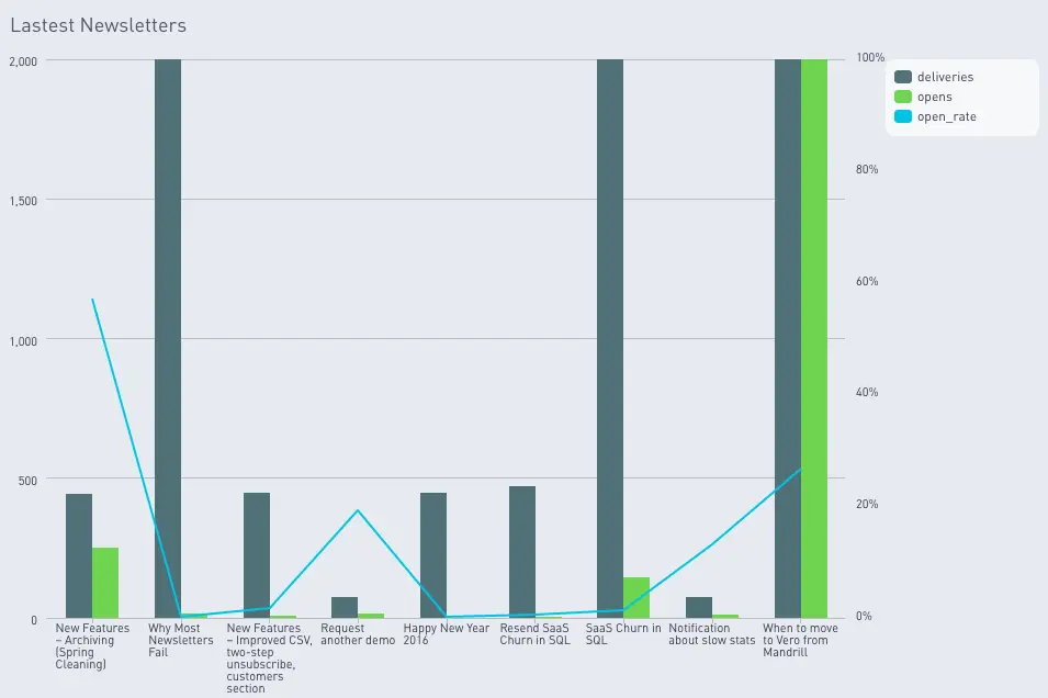
Charting open rates for your latest newsletter campaigns

Here’s an example of the chart we’ll be building.

What you’ll need to do this yourself

Here’s the setup we use to get accurate and complete data and to chart it beautifully:

• We use Vero to send all of Vero’s emails. Vero’s campaign management platform helps us create and manage our customer journey so we know who we’re sending what, and when. We send both automated and newsletter email campaigns with Vero.
• Segment’s integration automatically plugs into Vero and allows Vero to send back data on all email deliveries, opens, clicks, unsubscribes and so on into their platform.
• RJ Metrics’ Pipeline product syncs all of our Segment behavioral data to a Redshift database.
• Our data warehouse is hosted on a basic Amazon Web Services (AWS) Redshift cluster.
• We chart our reports using Periscope Data.
• We also use our own database with data about our users (in this case, we won’t be using this data, but we will in the future). Our application uses a mixture of datastores, but a PostgreSQL database contains the most relevant data.

This might sound complex, but all of these steps are a one to five-click process to get running. Once running, you have a really robust pipeline of user interaction data that you can use to build out sophisticated analyses any time you want.

Building your ‘deliveries’ and ‘opens’ data models

When you’re getting started with your SQL email analysis, the hardest part is getting your data in order.

The first step to creating the chart above is to create two SQL Views, one for your deliveries, and one for your opens. These views will represent a nice, clean view of all opens and all deliveries in your datastore, transformed and filtered to remove any junk. We’ll then use these tables to build out our charts.

Let’s dive into deliveries first.

Using the setup described above, your email data sends up in a Redshift database table via Segment. This is part of a large table called track, representing every user action that you have tracked via Segment (note: this includes any on-site activity, not just email deliveries).

For this analysis, create an SQL view called vero_analysis_deliveries_base. As you can see, this will view returning all of the raw fields you need for your analysis.

create or replace view vero_analysis_deliveries_base as (

  select 
    veroproduction.track.event                        as event,
    veroproduction.track.user_id                      as user_id,
    veroproduction.track.context__traits__email       as context__traits_email,
    veroproduction.track.properties__campaign_name    as properties__campaign_name,
    veroproduction.track.properties__email_subject    as properties__email_subject,
    veroproduction.track.properties__email_type       as properties__email_type,
    veroproduction.track.timestamp                    as timestamp
  from 
    veroproduction.track
    
);

This view can now be queried anytime and has only the data you need to create your email analysis charts.

The next step is to create an SQL view called vero_analysis_deliveries_filtered. In this view, select everything from the previous view, and filter out anything you don’t need. In this case we don’t want to filter anything, but it’s worth highlighting this step to help you learn to structure your data better.

create or replace view vero_analysis_deliveries_filtered as (

  select 
    *
  from 
    vero_analysis_deliveries_base
  where
    vero_analysis_sent_base.event = 'Email Delivered'
  and
    vero_analysis_deliveries_base.timestamp is not null

);

At this point, these views include all the data we need to create our tables, so it’s time to transform and normalize the formats for various columns (such as date columsn).

In this case we only want to see Email Delivered events (not the other Segment events) so you’ll want to filter out any other data in the track table.

To do this, create a view called vero_analysis_deliveries_transformed. This table will select everything from the vero_analysis_deliveries_filtered table and transform various columns, like the received_at column, into a consistent format.

create or replace view vero_analysis_deliveries_transformed as (

  select 
    vero_analysis_deliveries_filtered.user_id                      as user_id,
    vero_analysis_deliveries_filtered.context__traits_email        as user_email,
    vero_analysis_deliveries_filtered.properties__campaign_name    as campaign_name,
    vero_analysis_deliveries_filtered.properties__email_subject    as campaign_subject,
    vero_analysis_deliveries_filtered.properties__email_type       as campaign_type,
    vero_analysis_deliveries_filtered.timestamp::timestamp         as date
  from 
    [vero_analysis_deliveries_filtered]
  order by 
    date desc
    
);

That’s it! This is the final view you need to do the analysis. At this point the data is accurate, clean and it has it’s columns formatted in a way that makes it easy to query any time.

Full credit to the wonderful Tristan Handy at RJMetrics for this approach.

Creating your chart

Now that you’ve got everything you need, you can begin charting.

To create the chart mentioned in this post you need to query a table that has three columns: campaign_name, deliveries (the number of emails that were delivered), opens (the number of emails that were opened) and open_rate (the percentage open rate).

Here’s the SQL to do this.

with latest_newsletters as (
  select 
    campaign_name,
    max(date) as date
  from  
    [vero_analysis_deliveries_transformed]
  where
    campaign_type = 'newsletter'
  and
    campaign_name not like '%CLONE%'
  group by
    campaign_name
  order by
    max(date) desc
  limit 10
),

opens as (
  select 
    campaign_name,
    count(user_email) as opens
  from
    [vero_analysis_opens_transformed]
  group by
     campaign_name
),

deliveries as (
  select 
    campaign_name,
    count(user_email) as deliveries
  from
    [vero_analysis_deliveries_transformed]
  group by
     campaign_name
)
  
select 
  opens.campaign_name,
  deliveries.deliveries,
  opens.opens,
  (opens.opens::decimal  / deliveries.deliveries::decimal) as open_rate
from
  opens
join
  deliveries
on
  opens.campaign_name = deliveries.campaign_name
where
  opens.campaign_name in (
    select 
      campaign_name
    from
      latest_newsletters
  )

What is presented here comprises of three key steps.

Firstly, this SQL creates a temporary table that returns only the top ten most recent newsletters that you’ve sent. It does this by looking at the deliveries table and, for each campaign (grouped by the campaign name), returns the time of the last (max) email that was delivered.

You can then order by this field and return just ten campaigns. It’s also important, for this example, to filter down just the newsletters and not other automated campaigns (since you’ll have data on all of your emails from Vero).

Secondly, this SQL creates temporary tables that count how many deliveries and opens there were per campaign_name. Each of these temporary tables is separate. They return just the campaign_name and the count for the type of interaction we’re looking at.

Finally, we combine the campaign_name and opens temporary tables to return the campaign_name, the count of emails delivered and the count of emails opened. As part of this step we can do some maths to return a decimal number representing the percentage of emails that were opened.

That’s it! The final output is a table that you can use to create the graph above.

I charted my example using a bar chart to help compare absolute opens with absolute deliveries. I then used a line chart to highlight large peaks in open rate on a second Y axis. This gives a clearer perspective of each metric.

Next steps

This post was just an appetizer. This is a very basic analysis of your email data and forms the basis for much more complex, useful and interesting analysis.

If this looks useful to you, check out Vero.

If you are a Vero user and want to learn more about how you can do this drop us an email and we’d love to talk about it.

Share your thoughts and ideas in the comments below! I’d love to see what sorts of analyses you’ve built!